

About Hydro Forecasts
Finding the Best Forecast for Your Local Watershed
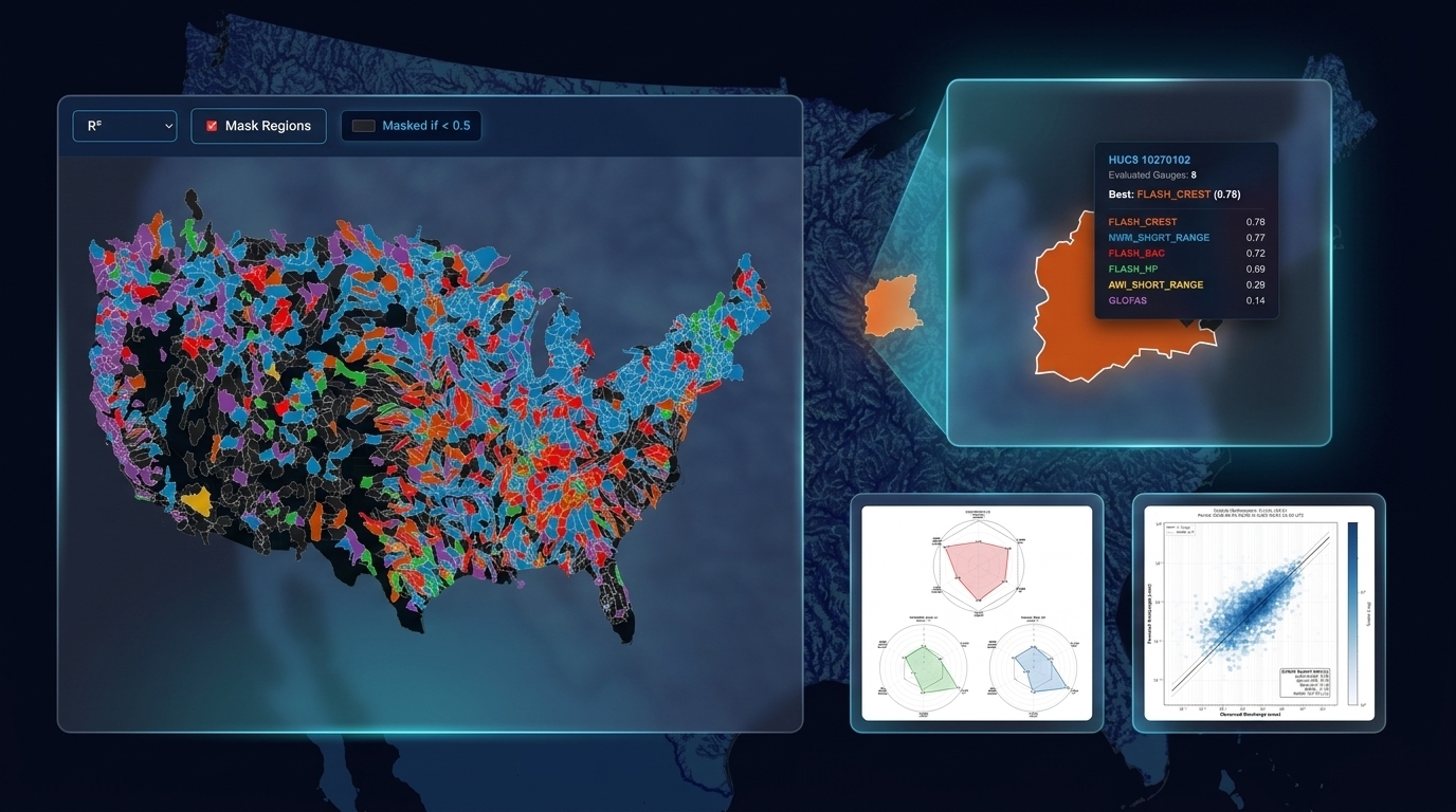
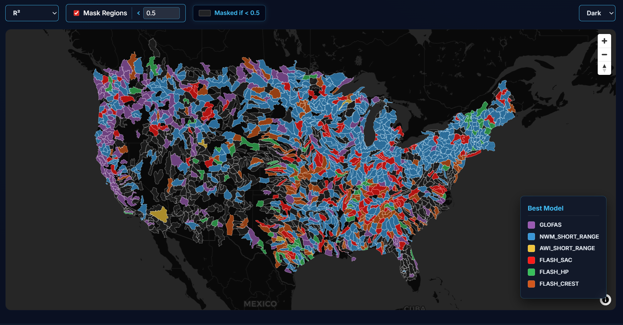
Imagine you are managing water resources or monitoring flood risks in a specific basin, such as HUC8 10190004 (the South Platte River). With half a dozen national models generating forecasts every few hours, deciding which one to trust can be overwhelming. Hydro Intel solves this by tracking the continuous 7-day historical performance of every model at every stream gauge. By navigating to the Score Cards tab and zooming in on your HUC8 polygon, you can instantly see which model (e.g., NWM Short Range or NOAA FLASH) yielded the highest median predictive skill (KGE or NSE) over the past week for your specific neighborhood.
Understanding Predictive Limits with the Model Skill Tab
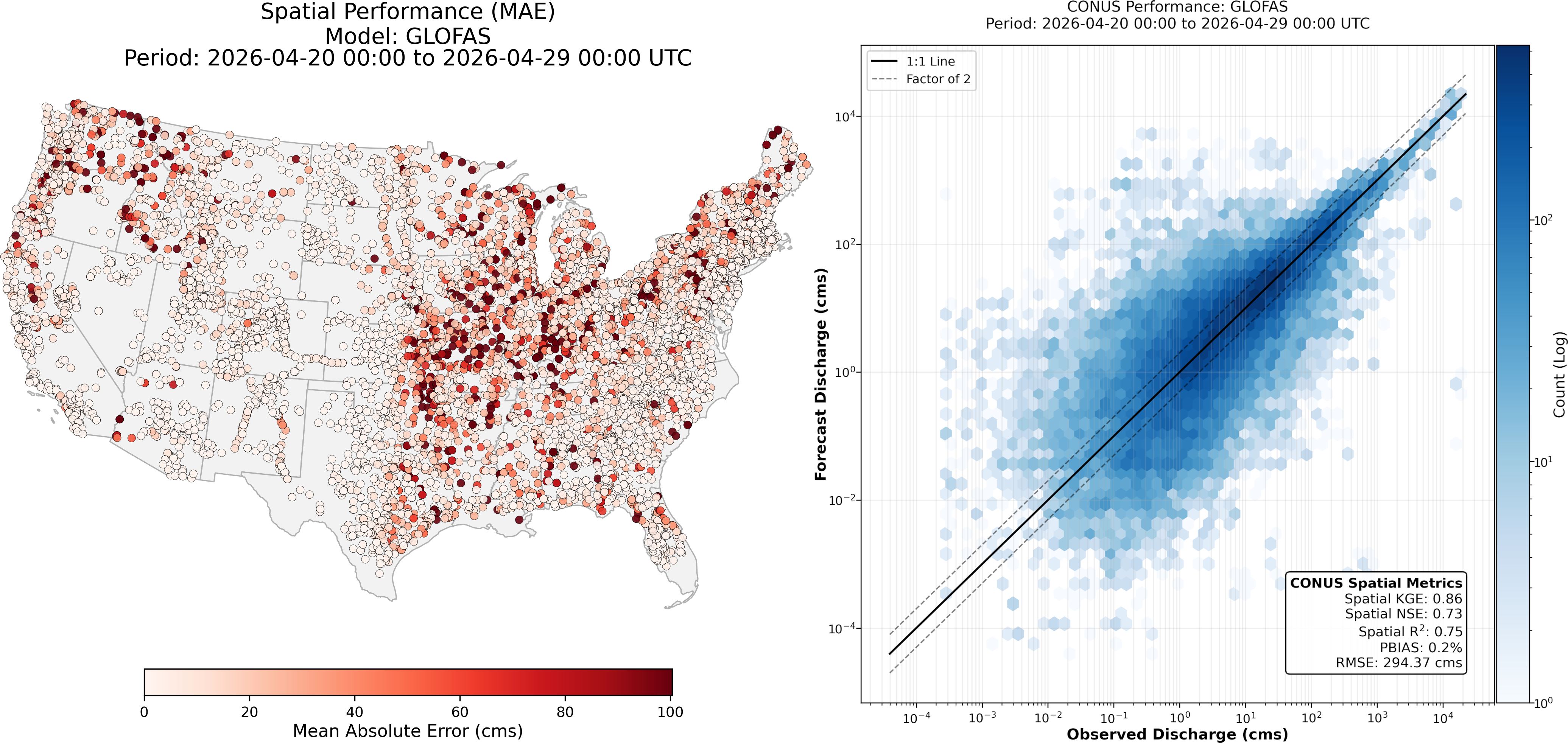
You can navigate to the Model Skill tab to evaluate a model’s overarching behavior during its most recent run. While the Score Card ranks localized, multi-day performance, the Model Skill tab provides an immediate, COntiguous United States (CONUS-wide) snapshot of a single, freshly completed forecast. By checking the national Observation vs. Simulation scatter plot, you can instantly spot systematic biases such as a universal tendency to underpredict major flood events. Meanwhile, the Spatial Error (MAE) map highlights exactly where across the country the model struggled or succeeded, providing critical context on how the model reacts to the current day's specific weather patterns.
Understanding how the Models behave
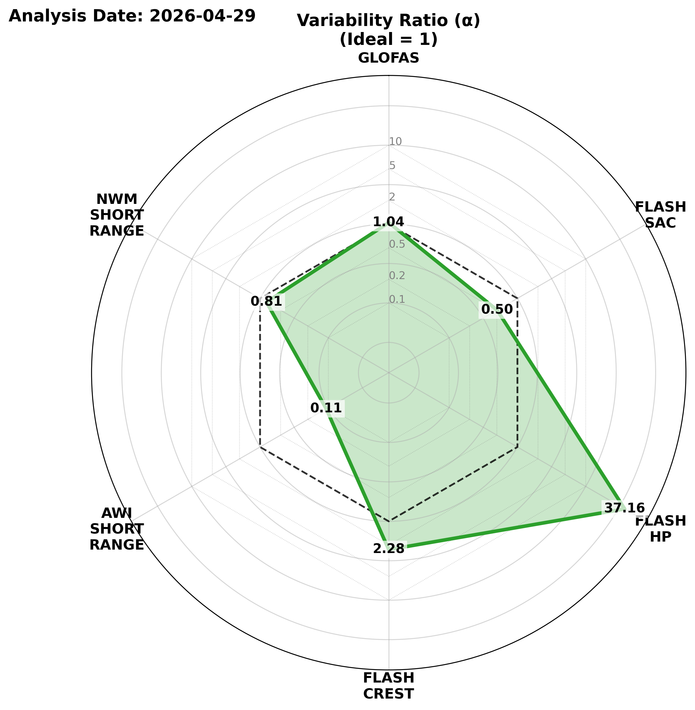
Once you know which model to look at, the KGE Decomposition Radar Plots tell you how to interpret its predictions. A high overall KGE score is great, but the radar charts break that score down into three critical behaviors: Correlation (r), Variability (α), and Volume Bias (β). If your region's winning model shows a perfect Correlation but a Volume Bias (β) of 1.2, it means the model is incredibly accurate at predicting exactly when the flood peak will arrive, but it tends to overpredict the total water volume by about 20%. This intelligence allows you to mentally adjust the forecast you are looking at.
Accessing Hydro Forecast Data
The Lynker Spatial data portal exposes key hydro-intelligence that is acaccessible programmatically using domain standard data standards such as zarr and parquet. We also provide more user-friendly access tools via the flowfabric-r or flowfabric-py packages, see the dedicated documentation pages within the individual package pages for more details.
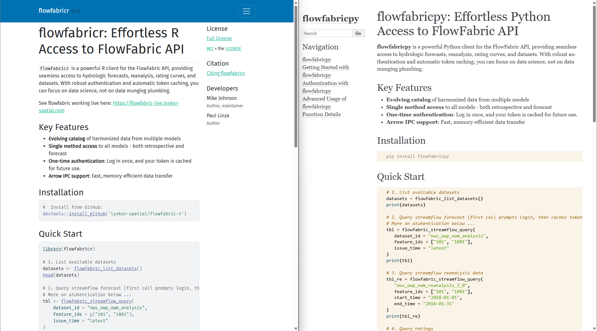
Below, we'll show you some of the most common access patterns exampling answers to common queries across the community.
Short Range (All)
import time
import xarray as xr
import dask

uri = "https://data.lynker-spatial.com/nwm/short_range/2025090214.zarr"

# Read Zarr metadata
start_metadata = time.time()
ds = xr.open_dataset(uri, engine="zarr", chunks="auto")
end_metadata = time.time()
#> 0.514 seconds

# Read Zarr data into memory from remote
start_memory = time.time()
ds_mem = ds.load()
end_memory = time.time()
#> 1.074 seconds

ds_mem
#> <xarray.Dataset> Size: 422MB
#> Dimensions:        (init_time: 1, forecast_time: 18, feature_id: 2776734)
#> Coordinates:
#>   * init_time      (init_time) datetime64[ns] 8B 2025-09-02T14:00:00
#>   * forecast_time  (forecast_time) datetime64[ns] 144B 2025-09-02T15:00:00 .....
#>   * feature_id     (feature_id) int64 22MB 101 179 181 ... 1180001803 1180001804
#> Data variables:
#>     streamflow     (init_time, forecast_time, feature_id) float64 400MB 0.17 ...
Short Range (Subset)
import time
import xarray as xr
import dask

reaches = [
    19305037,
    6965985,
    7099221,
    7718494,
    17168682,
    20073165,
    7558203,
    7318248,
    2330279,
    24423427
]

uri = "https://data.lynker-spatial.com/nwm/short_range/2025090214.zarr"
start = time.time()
ds = xr.open_dataset(uri, engine="zarr", chunks="auto")
#> <xarray.Dataset> Size: 422MB
#> Dimensions:        (init_time: 1, forecast_time: 18, feature_id: 2776734)
#> Coordinates:
#>   * init_time      (init_time) datetime64[ns] 8B 2025-09-02T14:00:00
#>   * forecast_time  (forecast_time) datetime64[ns] 144B 2025-09-02T15:00:00 .....
#>   * feature_id     (feature_id) int64 22MB 101 179 181 ... 1180001803 1180001804
#> Data variables:
#>     streamflow     (init_time, forecast_time, feature_id) float64 400MB 0.17 ...

ds = ds.where(ds.feature_id.isin(reaches), drop=True)
#> <xarray.Dataset> Size: 2kB
#> Dimensions:        (init_time: 1, forecast_time: 18, feature_id: 10)
#> Coordinates:
#>   * init_time      (init_time) datetime64[ns] 8B 2025-09-02T14:00:00
#>   * forecast_time  (forecast_time) datetime64[ns] 144B 2025-09-02T15:00:00 .....
#>   * feature_id     (feature_id) int64 80B 2330279 6965985 ... 20073165 24423427
#> Data variables:
#>     streamflow     (init_time, forecast_time, feature_id) float64 1kB 0.04 .....

ds = ds.load()
end = time.time()
#> 0.793 seconds
Short Range (Query)
import xarray as xr
import dask

uri = "https://data.lynker-spatial.com/nwm/short_range/2025090214.zarr"

# Read Zarr metadata
ds = xr.open_dataset(uri, engine="zarr", chunks="auto")

# Find 9 reaches where the streamflow exceeded 10 at least once
cond = (ds.streamflow > 10).compute()
reaches = ds.where(cond, drop=True).feature_id[:9]
ds = ds.sel(feature_id=reaches, drop=True)
ds_mem = ds.load()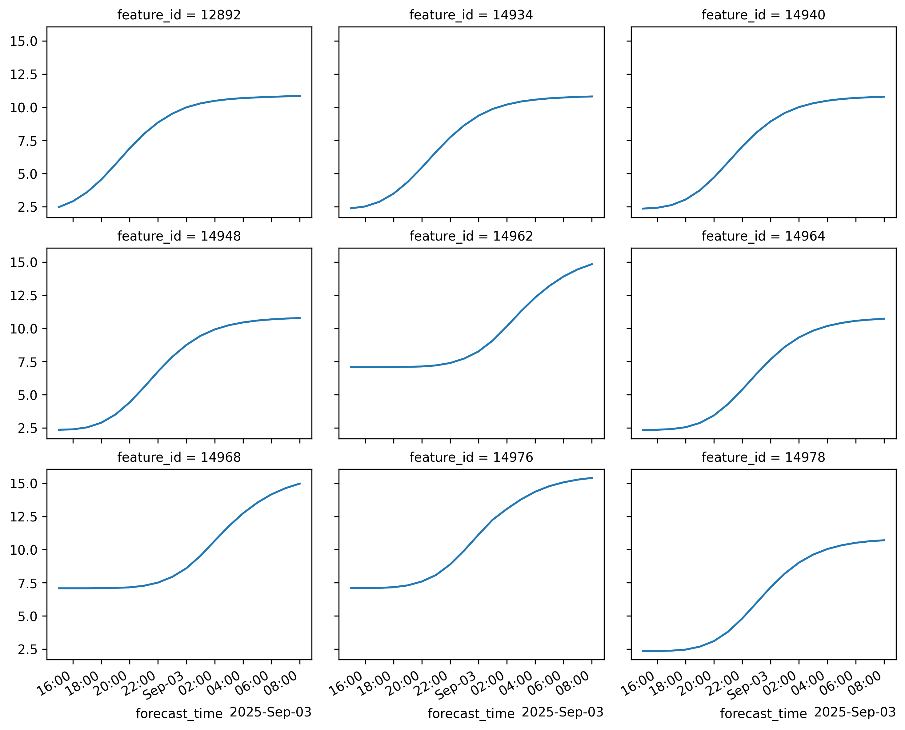
Analysis and Assimilation
uri = "https://data.lynker-spatial.com/nwm/analysis/2025090214.zarr"
start = time.time()
ds = xr.open_dataset(uri, engine="zarr", chunks="auto")
#> <xarray.Dataset> Size: 89MB
#> Dimensions:        (init_time: 1, forecast_time: 3, feature_id: 2776734)
#> Coordinates:
#>   * forecast_time  (forecast_time) datetime64[ns] 24B 2025-09-02T14:00:00 ......
#>   * init_time      (init_time) datetime64[ns] 8B 2025-09-02T14:00:00
#>   * feature_id     (feature_id) int64 22MB 101 179 181 ... 1180001803 1180001804
#> Data variables:
#>     streamflow     (init_time, forecast_time, feature_id) float64 67MB dask.array<chunksize=(1, 3, 2776734), meta=np.ndarray>

ds = ds.where(ds.feature_id.isin(reaches), drop=True)
#> <xarray.Dataset> Size: 352B
#> Dimensions:        (init_time: 1, forecast_time: 3, feature_id: 10)
#> Coordinates:
#>   * forecast_time  (forecast_time) datetime64[ns] 24B 2025-09-02T14:00:00 ......
#>   * init_time      (init_time) datetime64[ns] 8B 2025-09-02T14:00:00
#>   * feature_id     (feature_id) int64 80B 2330279 6965985 ... 20073165 24423427
#> Data variables:
#>     streamflow     (init_time, forecast_time, feature_id) float64 240B dask.array<chunksize=(1, 3, 10), meta=np.ndarray>

ds = ds.load()
end = time.time()
#> 3.0864 seconds
NWIS Observations
uri = "https://data.lynker-spatial.com/nwis/2025090214_discharge.zarr"
start = time.time()
ds = xr.open_dataset(uri, engine="zarr")
#> <xarray.Dataset> Size: 3MB
#> Dimensions:    (site_id: 8457, time: 61)
#> Coordinates:
#>     lon        (site_id) float64 68kB ...
#>     lat        (site_id) float64 68kB ...
#>   * site_id    (site_id) <U15 507kB '01010000' '01010070' ... '463836090423701'
#>     site_name  (site_id) object 68kB ...
#>   * time       (time) datetime64[ns] 488B 2025-09-02T14:00:00 ... 2025-09-02T...
#> Data variables:
#>     discharge  (site_id, time) float32 2MB ...
#> Attributes:
#>     source:        USGS NWIS Instantaneous Values (iv)
#>     window_start:  2025-09-02T14:00:00Z
#>     window_end:    2025-09-02T15:00:00Z
#>     aggregation:   last
#>     variables:     discharge(00060)


ds = ds.where(ds.site_id == "06752260", drop=True)
#> <xarray.Dataset> Size: 816B
#> Dimensions:    (site_id: 1, time: 61)
#> Coordinates:
#>     lon        (site_id) float64 8B -105.1
#>     lat        (site_id) float64 8B 40.59
#>   * site_id    (site_id) <U15 60B '06752260'
#>     site_name  (site_id) object 8B 'CACHE LA POUDRE RIVER AT FORT COLLINS, CO'
#>   * time       (time) datetime64[ns] 488B 2025-09-02T14:00:00 ... 2025-09-02T...
#> Data variables:
#>     discharge  (site_id, time) float32 244B 46.3 nan nan nan ... nan nan 46.3
#> Attributes:
#>     source:        USGS NWIS Instantaneous Values (iv)
#>     window_start:  2025-09-02T14:00:00Z
#>     window_end:    2025-09-02T15:00:00Z
#>     aggregation:   last
#>     variables:     discharge(00060)

ds = ds.load()
end = time.time()
#> 1.894 seconds